SiGN • SiGN

SiGN is an R package designed to streamline and automate the calculations required to generate behavioural predictions from the Signal for Good News (SiGN) model.

Background

Several decades ago, researchers discovered that operant contingencies can be arranged such that pigeons (Columba livia) reliably develop a preference for options that yield less food over those that provide more (Kendall, 1974). This behaviour—commonly referred to as “suboptimal” choice—results in a systematic reduction in overall food intake under controlled laboratory conditions.

The SiGN model explains this puzzling pattern (and other choice behaviours in concurrent-chains procedures) by proposing that choice is conditionally reinforced when stimuli signal a reduction in the delay to food.

For a detailed description of the model and its calculations, see Dunn et al. (2024).

Assumptions

This document is intended to illustrate the use of the R package, not explain the SiGN model and all its requisite background information.

To make effective use of this article and package, users are expected to have a foundational understanding of concepts such as …

Operant conditioning
Schedules of reinforcement
Concurrent and concurrent-chains procedures
Delay-reduction hypothesis
And, of course, …. The SiGN (Signal for Good News) model

If these and other related terms are unfamiliar, the explanations and R outputs provided by this document may be difficult to interpret.

Additionally, a working knowledge of R programming is assumed. The examples provided require comfort with vectorised functions, data manipulation, and interpreting model output.

Common Abbreviations

The following abbreviations are used throughout the package:

dur: duration (any units)
p: probability
il: initial link
tl: terminal link
tr: terminal reinforcement
dr: delay-reduction

FYI: In this context, terminal reinforcement refers to the stimulus delivered at the end of a chained schedule. While this is often a primary (unconditional) reinforcer such as food, the SiGN model does not require it to be so—it could also be a secondary (conditional) reinforcer. For this reason, the more general term terminal reinforcement is used by the package.

Installation

As the SiGN package is currently in development, the easiest way to install it is from GitHub using the pak package:

install.packages("pak")
pak::pak("jpisklak/SiGN")

Then load the package with:

library(SiGN)

Generating a Prediction

There are two steps to generating predictions using the SiGN model:

Use the choice_params() function to create a list of model parameters.
Pass this list to the SiGN() function to obtain predictions.

The SiGN model uses parameters from a concurrent-chains procedure to generate an a priori prediction of choice behaviour. While the required list of arguments can be created manually, the helper function choice_params() simplifies this process and includes built-in checks to ensure valid input.

Example: Stagner & Zentall (2010)

To illustrate, consider the contingencies described by Stagner and Zentall (2010), illustrated in Figure 1.

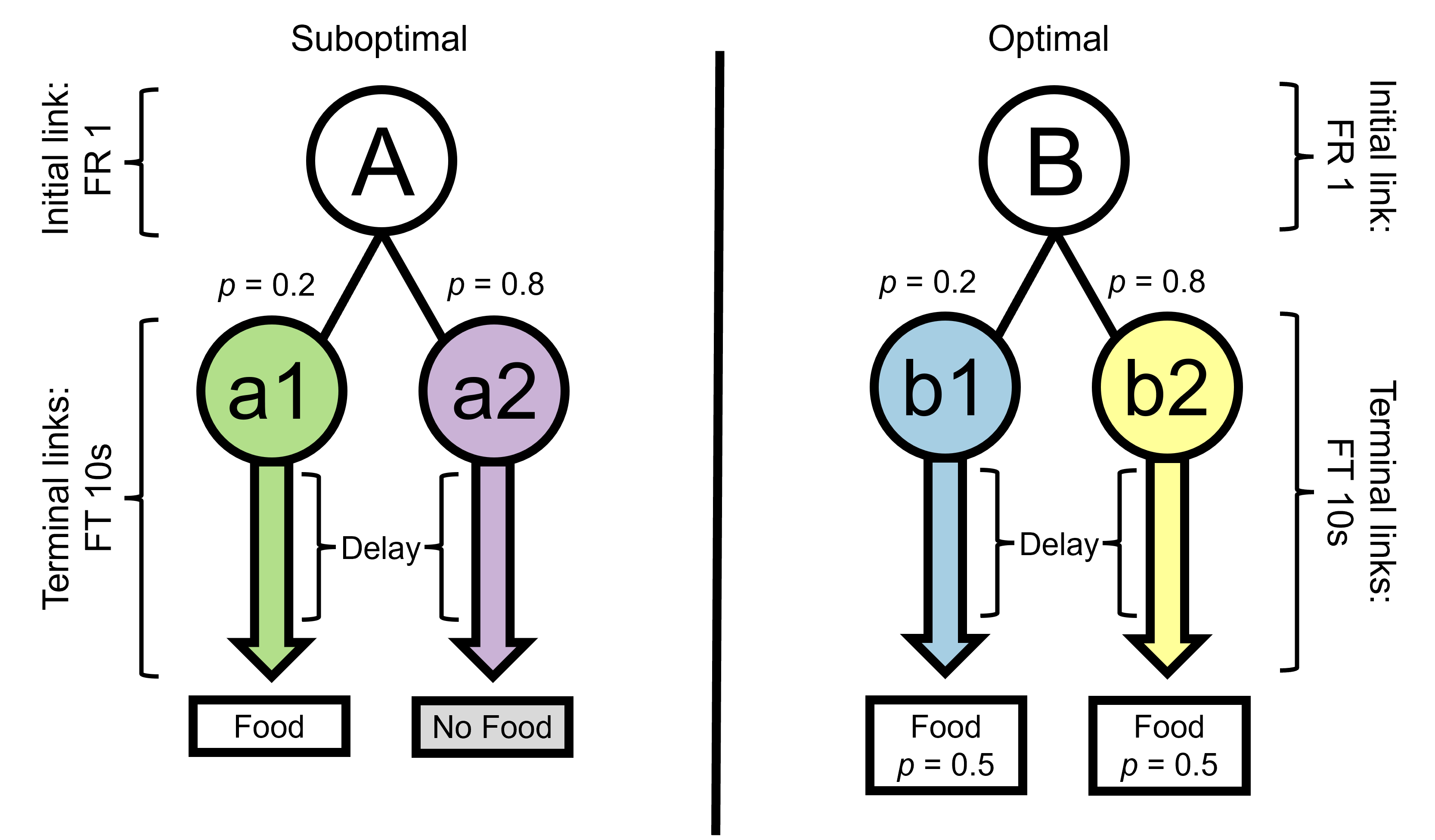
**Figure 1.** Stagner & Zentall (2010) contingencies

This procedure involves 16 distinct parameters, plus 2 additional parameters specific to the SiGN model—making a total of 18 values that need to be input into the SiGN() function. To speed up the process of entering these values, the choice_params() function includes several pre-defined profiles: "zentall" (Stagner & Zentall, 2010), "kendall" (Kendall, 1985), and "fantino" (Fantino, 1969).

The "zentall" profile matches the setup shown in Figure 1. You can view the full set of parameters by setting the argument display_params to be TRUE:

library(SiGN)
params <- choice_params("zentall", display_params = TRUE)
#>   il_dur_a il_dur_b tl_dur_a1 tl_dur_a2 tl_dur_b1 tl_dur_b2 tl_p_a1 tl_p_a2
#> 1        1        1        10        10        10        10     0.2     0.8
#>   tl_p_b1 tl_p_b2 tr_p_a1 tr_p_a2 tr_p_b1 tr_p_b2 il_sched_a il_sched_b s_delta
#> 1     0.2     0.8       1       0     0.5     0.5         FR         FR       1
#>   beta_log beta_toggle
#> 1       10        TRUE

The R documentation ?choice_params describes each parameter needed, but they are briefly listed in Table 1 below for convenience.

Table 1: Arguments for Model Parameters
Parameter	Description
`il_dur_a` `il_dur_b`	Initial link durations for alternative A and B.
`tl_dur_a1` `tl_dur_a2`	Durations for terminal links on A.
`tl_dur_b1` `tl_dur_b2`	Durations for terminal links on B.
`tl_p_a1` `tl_p_a2`	Entry probabilities for terminal links on A.
`tl_p_b1` `tl_p_b2`	Entry probabilities for terminal links on B.
`tr_p_a1` `tr_p_a2`	Reinforcement probabilities for terminal links on A.
`tr_p_b1` `tr_p_b2`	Reinforcement probabilities for terminal links on B.
`il_sched_a` `il_sched_b`	Initial link schedule types (“VI” or “FR”).
`s_delta`	Time to perceive a signal for no reinforcement. Default = 1.
`beta_log`	A positive real number specifying the base of the logarithm used for $\beta$.
`beta_toggle`	Logical toggle to disable $\beta$.

In most cases, s_delta does not require user modification (see the choice_params() documentation for exceptions). The arguments beta_log and beta_toggle influence the SiGN model’s $\beta$ parameter but are supplied automatically by the function and are not intended for direct user manipulation.

Once you have your parameter list, you can generate a prediction by passing it to the SiGN() function:

mod <- SiGN(params)
mod
#> Predicted Choice Proportion:
#> [1] 0.9590059
#> 
#> Use `$details` for additional model terms.

From the output, we can see that alternative A (the “suboptimal” alternative) will be selected approximately 96% of the time. To extract additional model details:

mod$details
#>          cp        r_a        r_b r_a_com r_b_com    Big_T     cr_a      cr_b
#> 1 0.9590059 0.05263158 0.04545455      NA      NA 21.14286 11.54496 0.5714286
#>   dr_avg_a  dr_avg_b dr_bonus_a dr_bonus_b   beta_a beta_b sig_a sig_b tr_p_a
#> 1 1.428571 0.5714286   9.714286          0 1.041393      1  TRUE FALSE    0.2
#>   tr_p_b s_delta beta_log
#> 1    0.5       1       10

An in-depth explanation of the $details output is beyond the scope of this document. Readers interested in the theoretical rationale behind these terms are referred to Dunn et al. 2024. However, a brief description of each component is provided in Table 2 below.

Table 2: Components of the `SiGN()` Function Output (`$details`)
Name	Description	Dunn et al.
cp	Predicted proportion of choices made to alternative A.	$\frac{R_a}{R_a + R_b}$
r_a r_b	Rate of terminal reinforcement on each alternative.	$r_x$
r_a_com r_b_com	Reinforcement rate on each alternative using a common effective initial link duration (when both IL schedules are VI).
Big_T	Overall average time to terminal reinforcement from the onset of initial links.	$T$
cr_a cr_b	Conditional reinforcement for each alternative (i.e., total delay-reduction).	$\delta_x$ or $D_\text{total}$
dr_avg_a dr_avg_b	Average delay reduction on each alternative.	$D_\text{avg}$
dr_bonus_a dr_bonus_b	Bonus delay reduction (when one TL offers a stronger signal).	$D_\text{bonus}$
beta_a beta_b	Adjustment factor reflecting the balance of conditional vs. terminal reinforcement.	$\beta_x$
sig_a sig_b	Logical indicator of whether each alternative is considered signalled (see `?sig_check`).
tr_p_a tr_p_b	Overall terminal reinforcement probability on each alternative.
s_delta	The `s_delta` value passed to the `SiGN()` function.
beta_log	The logarithm base for $\beta$ passed to the `SiGN()` function.

Generating Multiple Predictions

The SiGN() function supports vectorised input, allowing users to generate multiple predictions simultaneously. This is particularly useful for examining how predicted choice changes as a function of a single parameter while holding others constant.

As an example, suppose we want to evaluate how increasing the duration of the initial links affects choice behaviour. This can be done by supplying a sequence of values to the il_dur_a and il_dur_b arguments in choice_params(). The rest of the parameters will remain fixed according to the "zentall" profile, while these two are overridden.

# Generate list of parameters
il_preds <- choice_params("zentall",
  il_dur_a = seq(1, 100, by = 0.01),
  il_dur_b = seq(1, 100, by = 0.01)
)

# Generate predictions
mod_il <- SiGN(il_preds)

# Plot predictions
plot(il_preds$il_dur_a, mod_il$cp,
  type = "l", lwd = 3.5, lty = 1,
  las = 1,
  xlim = c(0, 100), ylim = c(0, 1),
  xaxt = "n",
  xlab = "Duration of Initial Links in Seconds",
  ylab = "Suboptimal Choice Proportion"
)
axis(1, at = c(1, seq(10, 100, 10)))
abline(h = 0.5, lwd = 1, lty = 3, col = "grey")

This approach can be extended to explore the effects of any parameter (or combination of parameters) on predicted choice. Internally, the function will recycle or align vector lengths as needed, but users should verify that values are as they intended to avoid any unexpected behaviour.

References

Dunn, R. M., Pisklak, J. M., McDevitt, M. A., & Spetch, M. L. (2024). Suboptimal choice: A review and quantification of the signal for good news (SiGN) model. Psychological Review. 131(1), 58-78. https://doi.org/10.1037/rev0000416

Fantino, E. (1969). Choice and rate of reinforcement. Journal of the Experimental Analysis of Behavior, 12(5), 723–730. https://doi.org/10.1901/jeab.1969.12-723

Kendall, S. B. (1974). Preference for intermittent reinforcement. Journal of the Experimental Analysis of Behavior, 21(3), 463–473. https://doi.org/10.1901/jeab.1974.21-463

Kendall, S. B. (1985). A further study of choice and percentage reinforcement. Behavioural Processes, 10(4), 399–413. https://doi.org/10.1016/0376-6357(85)90040-3

Stagner, J. P., & Zentall, T. R. (2010). Suboptimal choice behavior by pigeons. Psychonomic Bulletin & Review, 17(3), 412–416. https://doi.org/10.3758/PBR.17.3.412

Name	Description	Dunn et al.
cp	Predicted proportion of choices made to alternative A.	\(\frac{R_a}{R_a + R_b}\)
r_a r_b	Rate of terminal reinforcement on each alternative.	\(r_x\)
r_a_com r_b_com	Reinforcement rate on each alternative using a common effective initial link duration (when both IL schedules are VI).
Big_T	Overall average time to terminal reinforcement from the onset of initial links.	\(T\)
cr_a cr_b	Conditional reinforcement for each alternative (i.e., total delay-reduction).	\(\delta_x\) or \(D_\text{total}\)
dr_avg_a dr_avg_b	Average delay reduction on each alternative.	\(D_\text{avg}\)
dr_bonus_a dr_bonus_b	Bonus delay reduction (when one TL offers a stronger signal).	\(D_\text{bonus}\)
beta_a beta_b	Adjustment factor reflecting the balance of conditional vs. terminal reinforcement.	\(\beta_x\)
sig_a sig_b	Logical indicator of whether each alternative is considered signalled (see `?sig_check`).
tr_p_a tr_p_b	Overall terminal reinforcement probability on each alternative.
s_delta	The `s_delta` value passed to the `SiGN()` function.
beta_log	The logarithm base for \(\beta\) passed to the `SiGN()` function.